HOW-TO Perform a trend analysis and to find outliers
Summary
This HOW-TO shows how one can do a simple database trend analysis from the awe-prompt. In general to get to a result you need to do the following steps:
- Which quantities do you want to do a trendanalysis on? Determine which classes and attributes of objects in AWE are needed to get the desired information for those quantities.
- Construct the database query/queries required to get the desired information.
- Make a plot of the desired information to graphically detect outliers.
- Refine the constraints in the query to encompass only outliers.
- Retrieve the outlying objects and inspect them.
Examples
awe> q = (RawBiasFrame.chip.name == 'ccd50')
awe> biases = list(q)
awe> x = [b.MJD_OBS for b in biases]
awe> y = [b.imstat.median for b in biases]
awe> pylab.scatter(x,y,s=0.5)
This results in the plot in Figure 1 (zoomed, labels added).
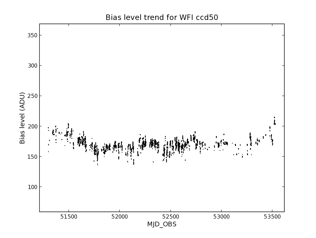
Figure 1: Trend analysis: bias level for all raw biases of CCD against modified julian date of observation.
awe> q = (RawBiasFrame.filename.like('WFI.2004*_1.fits'))
awe> len(q)
419
awe> biases = list(q)
awe> x = [b.MJD_OBS for b in biases]
awe> y = [b.imstat.median-b.overscan_x_stat.median for b in biases]
awe> pylab.scatter(x,y,s=0.5)
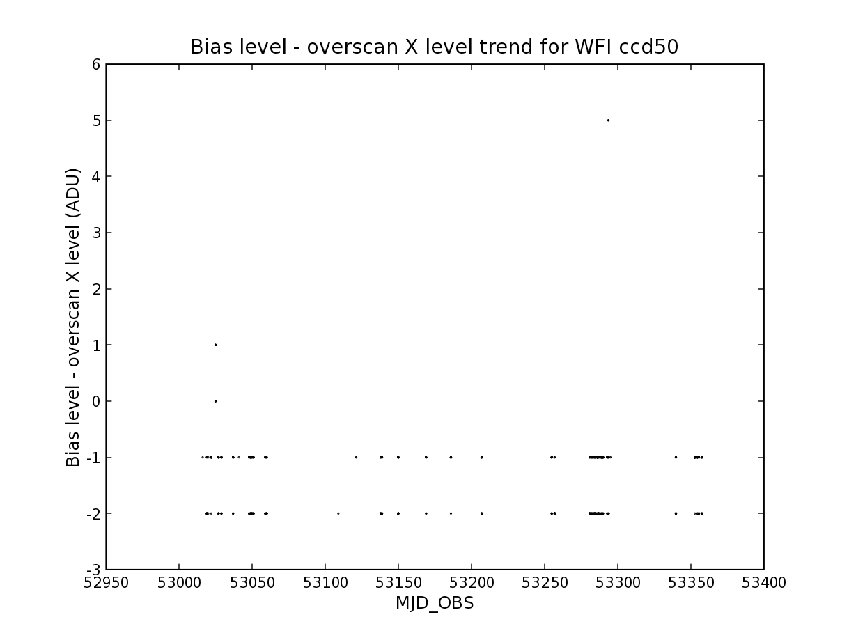
Figure 2: Trend analysis: trend of raw bias level in trim section minus the level in the overscan X region. The difference is plotted as a function of modified julian date of observation.
This produces a plot as in Figure 2. You can see that there seems to be one case where the difference is 5 ADU. This image will be interesting to look at. We can select it as follows:
awe> frames = [b for b in biases if b.imstat.median-b.overscan_x_stat.median > 4]
awe> len(frames)
2
awe> for f in frames: print(f.filename)
...
WFI.2004-10-15T15:10:02.248_1.fits
WFI.2004-10-15T15:11:52.384_1.fits
awe> for f in frames: f.retrieve()
...
It turns out there are in fact two frames of this kind. The images seem to have an uncharacteristic bright region in them; something was obviously wrong during these observations.