HOW-TO Image pipeline: overview
The image pipeline is the part of the system that processes science data. In this section, the image pipeline is discussed. A summary is given of the atomic tasks that make up the pipeline, and their place therein is described. Also given is an overview of how the image pipeline as a whole can be steered through the DPU interface. For the interface and use of every individual task, please read the corresponding HOW-TO.
The atomic tasks and their context
The atomic tasks that make up the image pipeline are summarized in Table 1, together with their role in the system and the identifier under which these are known to the DPU interface.
The sequence of tasks that make up the image pipeline is shown in Figure 1. In this figure, each one of the individual tasks is represented by one box. The arrows indicate the flow of the pipeline, and the shaded part shows a particular (optional) branch therein.
Contrary to the calibration pipelines, the start and end points of the image pipeline are flexible; one can choose to only de-bias and flatfield the data, but it is also possible to run the full pipeline including the global astrometry. The exception is the photometric calibration which has to be done separately. This requires performing Reduce, Astrometry and Photometry on a raw science frame of a standard star field. The resulting photometric parameters are then applied to the science image during the Regrid process.
Astrometry in the image pipeline
The astrometry in the image pipeline can be done in one of two ways. The first, and default, way is the traditional single-chip astrometry. This path through the image pipeline is shown in black in Figure 1. A more elaborate way of deriving the astrometric calibration is by combining the data of overlapping images to get a more accurate result for the single chips. This particular branch in the image pipeline, and the various tasks performed therein, is shown in light grey. Note that this branch augments the image pipeline, it does not supersede it.
Table 1: The various atomic processing steps that make up the image pipeline and the identifiers through which these can be selected by the user from the DPU interface
| Processing step | Purpose | DPU identifier |
|---|---|---|
| Reduce | De-biasing and flatfielding | Reduce |
| Astrometry | Single-chip astrometry | Astrometry |
| Photometry | Photometric calibration | Photom |
| Regrid | Regridding pixel data | Regrid |
| Coadd | Coadding pixel data | Coadd |
| GAstromSourceList | Making a sourcelist for global astrometry | GAstromSL |
| GAstrom | Deriving the global astrometry | GAstrom |
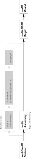
Figure 1: The order and flow of the atomic processing steps in the image processing part of the system. The lightly shaded part shows the (optional) branch into the global astrometry.
Running the image pipeline with the DPU
There are three ways in which the image pipeline can be run through the DPUinterface: (1) one task at a time, (2) using a pre-defined sequence without global astrometry, (3) using a pre-defined sequence with global astrometry.
The first way of running the image pipeline is simple: provide the DPU interface with one task identifier (see Table 1) and the appropriate query parameters. Example:
awe> dpu.run('Reduce', i='WFI',
             raw_filenames=['WFI.2000-04-29T00:40:57.671_1.fits'])
which will result in only de-biasing and flatfielding the selected frame. Another example:
awe> dpu.run('Reduce', i='WFI',
             raw_filenames=['WFI.2000-04-28T23:06:49.353_1.fits'])
which will result in determining photometric parameters, such as zeropoint and extinction coefficient, based on the standard star field frame ‘WFI.2000-04-28T23:06:49.353_1.fits’.
Besides this simple way of steering the image pipeline, it is also possible to provide the DPU interface with an identifier that selects a whole pre-defined sequence of tasks. The present set of pre-defined sequences (with and without global astrometry) is given in Table 2. All these sequences define ‘sane’ image pipelines that are internally consistent.
The identifiers given in Table 2 have the following structure:
(starting point of the pipeline)>(end point of the pipeline),
which will yield a traditional image pipeline with only single-chip astrometry. If one wants to include the global astrometry in the reduction, the structure is modified as follows:
(starting point of the pipeline)>GAstrometry>(end point of the pipeline),
where the extra GAstrometry clause explicitly instructs the image pipeline to switch to the global astrometry branch (the grey branch in Figure 1).
Table 2: The pre-defined sequences of image pipeline processing steps and their identifiers for the DPU interface. Note the way in which the global astrometry is enabled.
| Processing steps | DPU identifier |
|---|---|
| Reduce+Astrometry | Reduce>Astrometry |
| Reduce+Astrometry+Regrid | Reduce>Regrid |
| Reduce+Astrometry+Regrid+Coadd | Reduce>Coadd |
| Reduce+(GAstrometry)+Regrid | Reduce>GAstrometry>Regrid |
| Reduce+(GAstrometry)+Regrid+Coadd | Reduce>GAstrometry>Coadd |
| Regrid+Coadd | Regrid>Coadd |
Examples of using pre-defined sequences of tasks
Run the complete image pipeline all the way from de-biasing and flatfielding up to and including co-addition, but without global astrometry:
awe> dpu.run('Reduce>Coadd', instrument='WFI', date='2000-04-28',
             filter='#842', object='PG1525_B', commit=1)
Now do the same, but with global astrometry enabled (using short options this time):
awe> dpu.run('Reduce>GAstrometry>Coadd', i='WFI', d='2000-04-28', f='#842',
             o='PG1525_B', C=1)
Note that this particular sequence contains two processing steps that will be done on a single node, using results from the previous processing step.
Only de-biasing, flatfielding, and single-chip astrometry (for e.g. photometric standard fields):
awe> dpu.run('Reduce>Astrometry', i='WFI',
             raw_filenames=['WFI.2000-04-28T23:06:49.353_1.fits'])
Only de-biasing, flatfielding, single-chip astrometry, and regridding:
awe> dpu.run('Reduce>Regrid', i='WFI',
             raw_filenames=['WFI.2000-04-28T23:06:49.353_1.fits'])