HOW-TO Understand weights
The weighting scheme in the Astro-WISE system is relatively elaborate as a result of the regridding performed. In the course of the image pipeline (seq631-seq636 as described in the Data Flow System (.pdf)) 3 different weights may be constructed, the first weight is described in Science frames and their weight and the latter two are described in Weights created by SWarp.
Science frames and their weight
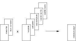
Individual weights
The science image is the end product of the pipeline for observations made in Stare mode, where no regridding operation is performed. Each science image has an associated weight.
The (normalized) flat-field describes the response of the telescope and instrument to a source of uniform radiation. In other words, it shows the relative amount of light received as a function of pixel position. This is a measure of the weight of a pixel relative to a pixel at a different position; the produced weights are relative weights.
Some pixels in an image are defect, counting too many or too few photons. These pixels are stored in hot- and cold pixel maps (values 1 for good, 0 for bad). In addition in a raw science image pixels may be unusable due to other causes. Pixel maps are created for saturated pixels, pixels affected by cosmic ray hits and pixels in satellite tracks. Saturated pixels are pixels whose counts exceed a certain threshold. In addition, saturation of a pixel may lead to ‘dead’ neighbouring pixels, whose counts lie below a lower threshold. Cosmic ray events can be detected using special source detections filters (retina filters), with SExtractor. These are essentially neural networks, trained to recognize cosmic rays, taking a set of neighbouring pixels as input. Satellite tracks can be discovered by a line-detection algorithm such as the Hough transform, where significant signal along a line produces a ‘peak’ in the transformed image. This peak can be clipped, and transformed back into a pixelmap that masks the track. The weight can therefore be written as:
It is possible that an illumination correction (photometric superflat) is used in the pipeline. As a result of stray light received by the detector the background of raw images is not flat. This effect is present both in science images and in flat-fields. In this case, dividing by the flat-field in the image pipeline results in a flat background, but in a non-uniform gain across the detector. In order to correct for this difference an illumination correction frame is made. This image is the result of the difference of the catalog magnitude of standard stars and their magnitude measured on reduced science frames, as a function of pixel position. The illumination correction can be viewed as a correction on the (incorrect) flat-field. Correctly applying the illumination correction therefore results in a non-flat background.
When an illumination correction is used the weight changes as follows:
In terms of our code base the object oriented class hierarchy for calibrated science images is shown below (specifying only relevant class dependencies):
ReducedScienceFrame                 (seq632)
  +-RawScienceFrame                 (seq631)
  +-MasterFlatFrame                 (req546)
  +-BiasFrame                       (req541)
  +-FringeFrame                     (req545)
  +-IlluminationCorrectionFrame     (req548)
  +-WeightFrame                     (seq633)
      +-MasterFlatFrame             (req546)
      +-IlluminationCorrectionFrame (req548)
      +-ColdPixelMap                (req535)
          +-DomeFlatFrame           (req535)
      +-HotPixelMap                 (req522)
          +-BiasFrame               (req541)
      +-SaturatedPixelMap
          +-RawScienceFrame
      +-CosmicMap
          +-RawScienceFrame
          +-HotPixelMap
          +-ColdPixelMap
          +-SaturatedPixelMap
          +-MasterFlatFrame
          +-IlluminationCorrectionFrame
      +-SatelliteMap
          +-RawScienceFrame
          +-HotPixelMap
          +-ColdPixelMap
          +-SaturatedPixelMap
          +-MasterFlatFrame
          +-IlluminationCorrectionFrame
Weights created by SWarp
Image coaddition is divided in two parts, resampling and combination. Image resampling addresses the problem that two independent observations of the same area of sky will, in general, result in images whose coordinate systems are different. Projection of these coordinate systems to a new coordinate system requires a mapping \(x,y \Rightarrow \alpha,\delta \Rightarrow x',y'\). Since the area of sky covered by an input pixel will in general not map directly to an area of sky covered by a single output pixel, some sort of interpolation is required. Unfortunately interpolation will inevitably result in aliasing artifacts, hence, a careful choice of interpolation kernel is required.
Once all input images and their weights have been resampled onto the grid specified by the coordinate system of the coadded image, it is straightforward to compute the coadded image and its weight. Given resampled input images \(1 \le i \le N\) entering co-addition, one can define for each pixel \(j\):
- the local uncalibrated flux \(f_{ij} = \overline{f_{ij}}+\Delta f_{ij}\), where \(\overline{f_{ij}}\) is the sky background, and \(\Delta f_{ij}\) the contribution from celestial sources,
- the local uncalibrated variance \(\sigma_{ij}^2 = \overline{\sigma_{ij}^2}+\Delta\sigma_{ij}^2\), where \(\overline{\sigma_{ij}^2}\) is background noise and \(\Delta\sigma_{ij}^2\) the photon shot noise of celestial sources,
- the local, normalized weight \(w_{ij}\),
- the electronic gain of the CCD \(g_i\),
- the relative flux scaling factor \(p_i\), deduced from the photometric solution, with \(p_i\Delta f_{ij} = p_l \Delta f_{lj}\) for all \(i,l,j\),
- the weight scaling factor \(k_i\).
Optimal weighting is obtained using
leading to a co-added flux (assuming the background of the input images has been subtracted),
and variance
The software package SWarp, developed by E. Bertin (IAP) for Terapix provides a set of regridding and co-addition algorithms specifically optimized to handle large area CCD mosaics.
Regridded frames and their weights
Whenever a calibrated science image is created in Dither mode (seq635) it is resampled to one of a number of pre-defined field centers (part of seq636). This affects both the science and weight images.
The default configuration of Swarp for making RegriddedFrames and their weights results in weight frames that are the resampled weight frame of the ReducedScienceFrame multiplied by \(1/\sigma^2\), where \(\sigma^2\) is the variance of the local background in units \({\rm ADU}^2\).
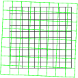
Regridded weights
The class hierarchy for regridded images is as follows:
RegriddedFrame
  +-AstrometricParameters
  +-PhotometricParameters
  +-ReducedScienceFrame
      +-(see section 1)
  +-WeightFrame           (produced by SWarp)
Coadded frames and their weights
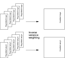
Coadded weights
When a collection of the regridded images described in the previous section are coadded a new weight is constructed by adding the (regridded) weights. In this step variance weighting is used to get a total weight.
The default configuration of Swarp for making CoaddedRegriddedFrames and their weights results in weight frames that contain the summation of the weights of the RegriddedFrames scaled by \(1/FLXSCALE^2\), where \(FLXSCALE^2\) is conversion factor from counts to the units of the CoaddedRegridded science frame. [1] Thus the weightframe is \(1/\sigma^2\), where \(\sigma^2\) is the variance of the local background with \(\sigma\) in the same units as the CoaddedRegriddedFrame science frame.
The class hierarchy for coadded frames is as follows:
CoaddedRegriddedFrame
  +-RegriddedFrame(s)
      +-(see section 2.1)
  +-WeightFrame       (produced by SWarp)
Weights in quality control
Three methods are defined for most calibration files, subdividing the quality control. The verify method is used to provide internal checks, often this takes the form of sanity checks on parameters of e.g. a BiasFrame. The compare method compares aspects of e.g. a BiasFrame (standard deviation for example) with that of a previous instance. Inspect is intended to show plots or images so that after an interactive analysis a decision can be made on the quality of the object.
In particular, statistics in subwindows of all images are used. While determining these statistics it is possible to provide a pixelmap of acceptable pixels. Below is a table that shows which weights/pixelmaps are (can be) used.
| Class | HotPixelMap | ColdPixelMap | SaturatedPixelMap | CosmicMap | SatelliteMap | Individual Weight |
|---|---|---|---|---|---|---|
| RawFrame | n | n | n | n | n | n |
| BiasFrame | n | n | n | n | n | n |
| DomeFlatFrame | y | y | n | n | n | n |
| TwilightFlatFrame | y | y | n | n | n | n |
| MasterFlatFrame | y | y | n | n | n | n |
| FringeFrame | y | y | n | n | n | n |
| ReducedScienceFrame | y | y | y | y | y | y |
| RegriddedFrame | n | n | n | n | n | y |
| [1] | TBD: is it the sum of each weightframe of a RegriddedFrame scaled with its own \(FLXSCALE\) (i.e., RegriddedFrame.FLXSCALE)? |